par(mfrow=c(1,3))
alpha = 4; beta = 1/2;
lambda = seq(0.1, 5, length.out = 50)
n_vals = c(10, 25, 50)
for(n in n_vals){
  mse_lambda_cap = lambda/n
  mse_lambdaB_cap = (beta^2*n*lambda + (alpha*beta-lambda)^2)/(n*beta+1)^2
  plot(lambda, mse_lambda_cap, col = "red", lwd=3, lty=1, type="l",
       xlab = expression(lambda), cex.lab = 1.2, ylab = "MSE", main = paste("n = ", n), cex.main = 1.5, cex.lab = 1.5)
  lines(lambda, mse_lambdaB_cap, col = "blue", lwd=3, lty=1)
  legend = c( expression(paste("MSE"[lambda], (hat(lambda)))),
              expression(paste("MSE"[lambda], (hat(lambda)[B]))))
  legend("topleft",legend = legend, lwd = c(3,3),col = c("red","blue"),
         lty = c(1,1), cex = 1, bty = "n")
  points(alpha*beta, 0, lwd=2, pch=20, cex=2)
}2 Illustrative Examples in practice
In this chapter, we will explore five commonly used examples in Bayesian inference. Each example is designed to show, step-by-step, how to calculate the posterior distribution, find the Bayesian estimate of the parameter, and compute the Mean Square Error (MSE) of the estimate.
These examples have been selected to clearly demonstrate how Bayesian methods work in practice for teaching purposes. By following these examples, one can gain a better understanding of how to apply Bayesian techniques and assess the accuracy of the estimates. The detailed calculations and used codes are included to make learning easier and more practical.
2.1 Example - I (Poisson rate parameter with gamma prior)
Let \(X_1, X_2,\cdots, X_n\) be a random sample of size \(n\) from a population following Poisson(\(\lambda\)) distribution. Suppose \(\lambda\) have a gamma(\(\alpha\), \(\beta\)) distribution, which is the conjugate family for Poisson. So, the statistical model has the following hierarchy:
\[\begin{eqnarray*} % \nonumber to remove numbering (before each equation) X_i|\lambda &\sim & \mbox{Poisson}(\lambda),~~i=1, 2,\cdots,n, \\ \lambda &\sim & \mbox{gamma}(\alpha,\beta). \end{eqnarray*}\]Based on the observed sample, we are interested to estimate the mean of the population, that is the value of \(\lambda\). The prior distribution of \(\lambda\), \(\pi(\lambda)\), is given by
\[\begin{equation*} \pi(\lambda) = \frac{\lambda^{\alpha-1}e^{-\frac{\lambda}{\beta}}}{\Gamma(\alpha) \beta^{\alpha}},~~\lambda>0, \end{equation*}\]where \(\alpha\) and \(\beta\) are positive constants. First, we shall obtain the posterior distribution of \(\lambda\). If there were no prior information available about the parameter \(\lambda\), then we could use the sample mean \(\overline{X}\) to estimate it. However, the exact sampling distribution of \(\overline{X}\) is not known in this case. Therefore, we begin with a statistic \(Y=\sum_{i=1}^nX_i\), whose sampling distribution is known to be Poisson(\(n\lambda\)) (denoted by \(f(y|\lambda)\)). The posterior distribution, the conditional distribution of \(\lambda\) given the sample, \(X_1, X_2,\cdots, X_n\), that is, given \(Y=y\), is
\[\begin{equation} \pi(\lambda|y) = \frac{f(y|\lambda)\pi(\lambda)}{m(y)}, \end{equation}\]where \(m(y)\) is the marginal distribution of \(Y\) and can be calculated as follows;
\[\begin{eqnarray*} % \nonumber to remove numbering (before each equation) m(y) &=& \int_0^{\infty}f(y|\lambda)\pi(\lambda)\mathrm{d}\lambda \\ &=& \int_0^{\infty}\frac{e^{-n\lambda}(n\lambda)^y}{y!}\cdot \frac{\lambda^{\alpha-1}e^{-\frac{\lambda}{\beta}}}{\Gamma(\alpha)\beta^{\alpha}}\mathrm{d}\lambda \\ &=& \frac{n^y}{y!\Gamma(\alpha)\beta^{\alpha}}\int_0^{\infty}e^{-\lambda\left(n+\frac{1}{\beta}\right)}\lambda^{y+\alpha -1}\mathrm{d}\lambda\\ &=& \frac{n^y \Gamma(y+\alpha)}{y!\Gamma(\alpha)\beta^{\alpha}\left(y+\frac{1}{\beta}\right)^{y+\alpha}}\int_0^{\infty}\frac{e^{-\lambda\left(n+\frac{1}{\beta}\right)}\lambda^{y+\alpha-1}\left(n+\frac{1}{\beta}\right)^{y+\alpha}}{\Gamma(y+\alpha)}\mathrm{d}\lambda\\ &=& \frac{n^y \Gamma(y+\alpha)}{y!\Gamma(\alpha)\beta^{\alpha}\left(n+\frac{1}{\beta}\right)^{y+\alpha}},~~y=0,1,2,\cdots. \end{eqnarray*}\]In the above, the integrand is the kernel of the \(\mbox{gamma}\left(y+\alpha, \left(n+\frac{1}{\beta}\right)^{-1}\right)\) density function, hence integrated out to be 1. Now, the posterior density \(\pi(\lambda|y)\) is given by \[\begin{eqnarray*} % \nonumber to remove numbering (before each equation) \pi(\lambda|y) &=& \frac{e^{-n\lambda}(n\lambda)^y}{y!}\cdot \frac{\lambda^{\alpha-1}e^{-\frac{\lambda}{\beta}}}{\Gamma(\alpha)\beta^{\alpha}}\ \cdot\frac{y!\Gamma(\alpha)\beta^{\alpha}\left(n+\frac{1}{\beta}\right)^{y+\alpha}}{n^y \Gamma(y+\alpha)}\\ & = & \frac{\left(n + \frac{1}{\beta}\right)^{y+\alpha}e^{-\lambda\left(n+\frac{1}{\beta}\right)}\lambda^{y+\alpha-1}}{\Gamma(y+\alpha)}, ~~0<\lambda <\infty. \end{eqnarray*}\] Hence, as expected, the posterior distribution of \(\lambda\), \[\lambda|y \sim \mbox{gamma}\left(y+\alpha, \left(n+\frac{1}{\beta}\right)^{-1}\right).\] It also verifies the claim that the gamma(\(\alpha\),\(\beta\)) is the conjugate family for Poisson. A closure look in the above calculations reveals that the steps can be heavily reduced, in fact the explicit expression for \(m(y)\) is not at all required. Since, it does not depend of \(\lambda\), it is a constant, that makes the integral \(\int_0^\infty \pi(\lambda|y)\mathrm{d}\lambda\) to be equal to 1, so that it becomes a valid probability density function. Thus, appearance of the posterior density in the integrand of the marginal is not a magic. We shall use this posterior distribution of \(\lambda\) to make statements about the parameter \(\lambda\). The mean of the posterior can be used as a point estimate of \(\lambda\). So, the Bayesian estimator of \(\lambda\) (call it \(\hat{\lambda}_B\)) is given by \(E(\lambda|Y)\). Because of the gamma density, we avoid the computation of the integral and directly write as: \[\begin{equation*} \hat{\lambda}_B = \frac{y+\alpha}{n+\frac{1}{\beta}} = \frac{\beta(y+\alpha)}{n\beta+1}. \end{equation*}\] Let us investigate the structure of the Bayesian estimate of \(\lambda\). If no data were available, we are forced to use the information from the prior distribution (only). \(\pi(\lambda)\) has the mean \(\alpha \beta\), which would be our best estimate of \(\lambda\). If no prior information were available, we would use \(Y/n\) (sample mean \(\overline{X}\)) to estimate \(\lambda\) and draw the conclusion based on the sample values only. Now, the beautiful part is that the Bayesian estimator combines all of these information (if available). We can write \(\hat{\lambda}_B\) in the following way. \[\begin{equation*} \hat{\lambda}_B = \left(\frac{n\beta}{n\beta+1}\right)\left(\frac{Y}{n}\right) + \left(\frac{1}{n\beta+1}\right)\left(\alpha \beta\right). \end{equation*}\] Thus \(\hat{\lambda}_B\) is a linear combination of the prior mean and the sample mean. The weights are determined by the values of \(\alpha\), \(\beta\) and \(n\).
Suppose that we increase the sample size such that \(n \to \infty\). Then \(\frac{n\beta}{n\beta+1} \to 1\) and \(\frac{1}{n\beta+1} \to 0\), and \(\hat{\lambda}_B \to \overline{X}\). The idea is that as we increase the sample size, the data histogram closely approximates the population distribution itself. As if we have got enough knowledge about the population itself (because of a large number of observations). Hence, the prior information becomes less relevant and the value of the sample mean dominates the Bayesian estimate of \(\lambda\). When the size of the sample is small, then it is wise to utilize the prior information about the population parameter. Hence, the term \(\left(\frac{\alpha \beta}{n\beta+1}\right)\) contributes significantly in the final estimate. By weak law of large numbers \(\overline{X} \to \lambda\) in probability as \(n\to \infty\), so \(\hat{\lambda}_B \to \theta\) in probability, proving that \(\hat{\lambda}_B\) is consistent estimator for \(\lambda\). Another interesting point is that, for any finite \(n\), \(\hat{\lambda}_B\) is a biased estimator of \(\lambda\), with \(\mbox{Bias}_{\lambda}(\hat{\lambda}_B) = \frac{\alpha \beta -\lambda}{n\beta + 1} \to 0\) as \(n\to \infty\). \(\hat{\lambda}_B\) is asymptotically unbiased.
We end up with two estimators for the parameter \(\lambda\), viz. Bayesian estimate, \(\hat{\lambda}_B\) and Maximum likelihood estimator \(\hat{\lambda} = \overline{X}\). It is natural to ask which estimator should we prefer? The efficiency of an estimator is computed by the Mean Square Error (MSE) which measures the average squared difference between the estimator and the parameter. In the present situation, the MSE of \(\hat{\lambda}\) is
\[\begin{equation*} \mbox{E}_{\lambda}(\hat{\lambda}-\lambda)^2 = \mbox{Var}_{\lambda}(\overline{X}) = \frac{\lambda}{n}. \end{equation*}\] Since, \(\overline{X}\) is an unbiased estimator of \(\lambda\), the MSE of \(\overline{X}\) is equal to its variance. Now, given \(Y=\sum_{i=1}^nX_i\), the MSE of the Bayesian estimator of \(\lambda\), \(\hat{\lambda}_B = \frac{\beta(Y+\alpha)}{n\beta +1}\), is
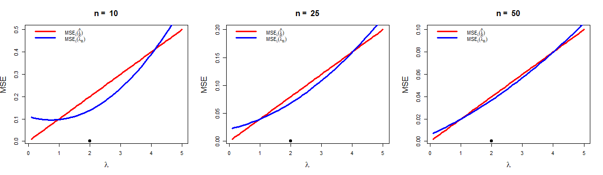
\[\begin{eqnarray*} % \nonumber to remove numbering (before each equation) \mbox{E}_{\lambda}(\hat{\lambda}_B-\lambda)^2 &=& \mbox{Var}_{\lambda}\hat{\lambda}_B + (\mbox{Bias}_{\lambda} \hat{\lambda}_B)^2\\ &=& \mbox{Var}_{\lambda}\left(\frac{\beta(Y+\alpha)}{n\beta +1}\right) + \left(\mbox{E}_{\lambda}\left(\frac{\beta(Y+\alpha)}{n\beta +1}\right)-\lambda\right)^2\\ &=& \frac{\beta^2 n\lambda}{(n\beta+1)^2} + \frac{(\alpha \beta -\lambda)^2}{(n\beta+1)^2}. \end{eqnarray*}\]For fixed \(n\), the above quantity will be minimum if \(\alpha\beta = \lambda\), that is the prior mean is equal to the true value. However, in general, MSE is a function of the parameter. So, it is highly unlikely that we would end up with a single estimator which is the best for all parameter values. In general the MSEs of two estimators cross each other. This demonstrates that one estimator is better with respect to another estimator in only a portion of the parameter space. Now let us delve deep further in comparing the above two estimators. If \(\lambda = \alpha \beta\), then for large \(n\), \[\mbox{MSE}_{\lambda}(\hat{\lambda}_B) = \frac{\beta^2 n\lambda}{(n\beta+1)^2} = \frac{\beta^2n\lambda}{n^2\beta^2\left(1+\frac{1}{n\beta}\right)^2} \approx \frac{\lambda}{n}.\] Thus, if the prior is chosen in a such way (choice of \(\alpha\) and \(\beta\)) so that the prior mean is close to the true value, then both the estimators have same variance approximately, for large \(n\). This observation is depicted in Figure 2.1. We consider the values of \(\alpha\) and \(\beta\) to be \(4\) and \(\frac{1}{2}\), respectively, so that the prior mean is \(\alpha \beta =2\). It is clear from the figure that if prior mean is close to the true value, then \(\hat{\lambda}_B\) performs better than \(\hat{\lambda}\). If the prior mean is much away from the true value, then \(\hat{\lambda}\) performs better than \(\hat{\lambda}_B\). However, for large sample size (\(n\to \infty\)) both the estimators have same MSE.
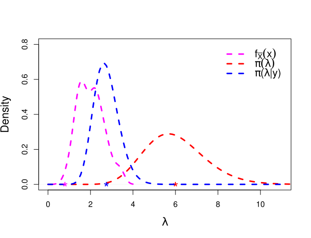
We have seen that the posterior mean is a linear combination of prior mean and the sample mean. Basically, the Bayesian estimate lies between the sample mean and prior mean. That is, the linear combination is in fact a convex combination. This can also be better visualized if we plot the three distributions in a single plot window, viz. the data histogram, prior distribution, posterior distribution (Figure 2.2).
R Code for Figure 2.1
R Code for Figure 2.2
par(mfrow=c(1,1))

# sampling distribution of sample mean
n = 5                                       # sample size
lambda = 2                                  # true mean values
set.seed(123)                               # reporducibility of simualtion
rep = 100                                   # number of replication
mean_vals = numeric(length = rep)
for(i in 1:rep){
    mean_vals[i] = mean(rpois(n = n, lambda = lambda))
}
plot(density(mean_vals), lwd=3, col = "magenta",  xlim = c(0, 11), ylim =c(0,.8), main = "",
    xlab = expression(lambda), cex.lab = 1.4, lty = 2)

# Prior density of lambda
alpha = 18; beta = 1/3                      # hyperparameters
prior_density = function(x){                # prior density
    exp(-x/beta)*x^(alpha-1)/(beta^alpha * gamma(alpha))
}
curve(prior_density(x), 0, 13, col = "red", lwd=3, add = TRUE, lty = 2)
points(alpha*beta, 0, lwd=2, col ="red", pch = "*", cex=2)

y = sum(rpois(n = n, lambda = lambda))      # sufficient statistic
posterior_density = function(x){            # posterior density
    (n+1/beta)^(y+alpha)*exp(-x*(n+1/beta))*x^(y+alpha-1)/gamma(y+alpha)
}
curve(posterior_density(x), col = "blue", lwd=3, add = TRUE, lty = 2)
points(beta*(y+alpha)/(n*beta + 1),0, lwd=2, col ="blue", pch = "*", cex=2)     # posterior mean
points(y/n, 0, lwd=2, col ="magenta", pch = "*", cex=2)
legend(8,0.8, c(expression(f[bar(X)](x)), expression(pi(lambda)),
                expression(paste(pi,"(",lambda, "|", y,")" ))),
lwd=rep(3,3), col = c("magenta", "red", "blue"),  bty="n", cex = 1.3, lty = rep(2, 3))
2.2 Example - II (Normal prior for normal mean)
Suppose we observe a sample of size 1, \(X \sim \mathcal{N}(\theta, \sigma^2)\) and suppose that the prior distribution of \(\theta\) is \(\mathcal{N}(\mu, \tau^2)\). We assume that the quantities, \(\sigma^2\), \(\mu\) and \(\tau^2\) are all known. We are interested to obtain the posterior distribution of \(\theta\). The prior distribution is given as;
\[\begin{equation*} \pi(\theta) = \frac{1}{\tau \sqrt{2\pi}}e^{-\frac{(\theta-\mu)^2}{2\tau^2}}, ~~-\infty<\mu, \theta <\infty,~0 <\tau<\infty. \end{equation*}\]The posterior density function of \(\theta\) is given as follows;
\[\begin{eqnarray*} \pi(\theta|x) &=& \frac{f(x|\theta)\pi(\theta)}{\int_{-\infty}^{\infty}f(x|\theta)\pi(\theta)\mathrm{d}\theta}\\ &=& \frac{\frac{1}{\sigma \tau (\sqrt{2\pi})^2}\exp\left\{-\frac{1}{2}\left[\left(\frac{x-\theta}{\sigma}\right)^2 + \left(\frac{\theta-\mu}{\tau}\right)^2\right]\right\}}{{\int_{-\infty}^{\infty}f(x|\theta)\pi(\theta)\mathrm{d}\theta}}. \end{eqnarray*}\]The exponent can be expressed as
\[\begin{equation*} \frac{\sigma^2 +\tau^2}{\sigma^2\tau^2}\cdot \left[\left(\theta - \frac{x\tau^2 + \mu \sigma^2}{\sigma^2 + \tau^2}\right)^2 + \frac{\tau^2 x^2 + \mu^2 \sigma^2}{\sigma^2 + \tau^2} - \left(\frac{x\tau^2 + \mu^2\sigma^2}{\sigma^2 + \tau^2}\right)^2\right]. \end{equation*}\]Note that, all the terms except containing the expression of \(\theta\) will be cancelled with the denominator, resulting the posterior density of \(\theta\) given as follows;
\[\begin{equation*} \pi(\theta|x) = \frac{\sqrt{\sigma^2 +\tau^2}}{\sigma\tau\sqrt{2\pi}}\exp\left[-\frac{\sigma^2 +\tau^2}{2 \sigma^2 \tau^2}\left(\theta - \frac{x\tau^2 + \mu \sigma^2}{\sigma^2 + \tau^2}\right)^2\right]. \end{equation*}\]The posterior distribution of \(\theta\) is normal, showing that the normal family is its own conjugate when indexed by the mean (\(\theta\)). The posterior mean and variance of \(\theta\) are as follows;
\[\begin{equation*} % \nonumber to remove numbering (before each equation) \mbox{E}(\theta|x) = \frac{x\tau^2 + \mu \sigma^2}{\sigma^2 + \tau^2},~~~~~\mbox{and}~~~~ \mbox{Var}(\theta|x) = \frac{\sigma^2 \tau^2}{\sigma^2 +\tau^2}. \end{equation*}\]As discussed earlier, \(\mbox{E}(\theta|x)\) is a point of estimate of \(\theta\), thus the Bayesian estimator of \(\theta\) based on a single sample is given by
\[\begin{equation*} \hat{\theta}_B = \frac{X\tau^2 + \mu \sigma^2}{\sigma^2 + \tau^2} = \left(\frac{\tau^2}{\sigma^2 + \tau^2}\right)X + \left(\frac{\sigma^2}{\sigma^2 + \tau^2}\right)\mu. \end{equation*}\]Again, the Bayesian estimate of \(\theta\) is a linear combination of the prior mean and the sample value (which is in fact the estimate of \(\theta\), as the size of the sample is 1). We shall treat this problem based on a sample of size \(n\) and obtain the Bayesian estimator of \(\theta\) using it. A tedious calculation is required to obtain the posterior distribution. However, that will help us to obtain the the distribution of \(\theta|\overline{X}\) easily. Suppose that we draw a sample \(X_1, X_2,\cdots,X_n\) of size \(n\) from \(\mathcal{N}(\theta,\sigma^2)\), then the sample mean \(\overline{X} \sim \mathcal{N}(\theta, \sigma^2/n)\). The same calculation will follow with \(X\) would be replaced by \(\overline{X}\) and \(\sigma^2\) will be replaced by \(\frac{\sigma^2}{n}\), respectively. Then the posterior distribution of \(\theta\) is normal, with mean and variance given by
\[\begin{equation*} \mbox{E}(\theta|\overline{x}) = \frac{\overline{x}n\tau^2 + \mu \sigma^2}{\sigma^2 + n\tau^2},~~~~~~~~~ \mbox{Var}(\theta|\overline{x}) = \frac{\sigma^2 \tau^2}{\sigma^2 +n\tau^2}, \end{equation*}\]and the Bayesian estimator is given as follows;
\[\begin{equation*} \hat{\theta}_B = \left(\frac{n\tau^2}{\sigma^2 + n\tau^2}\right)\overline{X} + \left(\frac{\sigma^2}{\sigma^2 + n\tau^2}\right)\mu. \end{equation*}\]As \(n\to \infty\), \(\frac{n\tau^2}{\sigma^2 + n\tau^2} \to 1\) and \(\frac{\sigma^2}{\sigma^2 + n\tau^2} \to 0\), so that \(\hat{\theta}_B \approx \overline{X}\). But, when \(n\) is small, use of prior information improves the estimate. Since, \(\overline{X}\to \theta\) in probability as \(n\to \infty\), which follows that \(\hat{\theta}_B \to \theta\) in probability as \(n\to \infty\) (By Slutsky’s theorem). MSE of \(\hat{\theta}_B\) is given by
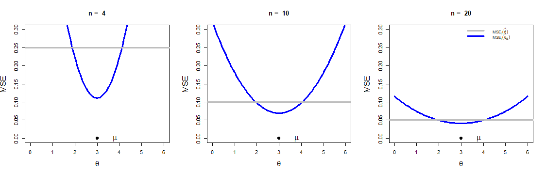
\[\begin{eqnarray*} % \nonumber to remove numbering (before each equation) \mbox{E}_{\theta}(\hat{\theta}_B - \theta)^2 &=& \mbox{Var}_{\theta}(\hat{\theta}_B) + \left(\mbox{Bias}_{\theta}(\hat{\theta}_B)\right)^2 \\ &=& \mbox{Var}_{\theta}\left(\frac{\overline{X}n\tau^2 + \mu \sigma^2}{\sigma^2 + n\tau^2}\right) + \left(\mbox{E}_{\theta}\left(\frac{\overline{X}n\tau^2 + \mu \sigma^2}{\sigma^2 + n\tau^2}\right)-\theta\right)^2\\ &=& \frac{\tau^4 n\sigma^2}{(\sigma^2 +n\tau^2)^2} + \left(\frac{(\mu-\theta)\sigma^2}{\sigma^2 +n\tau^2}\right)^2\\ &=& \frac{\sigma^2}{\left(\sigma^2+n\tau^2 \right)^2}\cdot\left(n\tau^4 + (\mu-\theta)^2\sigma^2\right). \end{eqnarray*}\]The estimators \(\hat{\theta}_B\) and \(\overline{X}\) are compared for different sample sizes and also for different choices of the prior variance \(\tau^2\) (Figure 4.2 (a) and Figure 4.2 (b)). The estimator can also be compared by using the relative efficiency, which is defined as the MSE of the two estimators. So the efficiency of \(\hat{\theta}_B\) relative to \(\overline{X}\), \(\mbox{eff}_{\theta}(\hat{\theta}_B|\overline{X})\), is
\[\begin{equation*} \frac{\mbox{MSE}_{\theta}(\hat{\theta}_B)}{\mbox{MSE}_{\theta}(\overline{X})} = \frac{n\tau^4 + (\mu-\theta)^2\sigma^2}{\left( \sigma^2 + n\tau^2\right)^2}. \end{equation*}\] If \(\mu = \theta\), for a given sample size \(n\), relative efficiency is minimum and less than 1. Hence, \(\hat{\theta}_B\) is more efficient than \(\overline{X}\) for any given \(n\). If we move \(\theta\) values away from \(\mu\), then \(\mbox{eff}_{\theta}(\hat{\theta}_B|\overline{X})\) crosses the line \(y=1\). For theta values beyond that point, \(\overline{X}\) is better than \(\hat{\theta}_B\). We encourage the reader to draw this picture and compare two estimators based on the relative efficiency. It is clearly understood that, essentially we are describing the same thing, only with a different graphical representation. Of course, the function \(\texttt{curve}\) from \(\texttt{R}\) is a very useful tool, which has been utilized throughout this material.

R Code for Figure 4.2 (a) and Figure 4.2 (b)
sigma = sqrt(1)     # population sd, known
mu = 3              # prior mean value
tau = sqrt(0.5)     # prior sd
n_vals = c(4, 10, 20) # sample size

par(mfrow=c(2,3))   # space for six plots in a single window
for(n in n_vals){
  curve(sigma^2/(sigma^2 + n*tau^2)^2*(n*tau^4 + (mu-x)^2*sigma^2),
        0, 6, col = "blue", lwd=3, ylab = "MSE", ylim=c(0,0.3),
        main = paste("n = ", n), xlab = expression(theta), cex.lab = 1.5)
  abline(h=sigma^2/n,col = "grey", lwd=3)
  points(mu, 0, lwd=2.5, pch=20, cex=2)
  text(mu+0.8, 0, expression(mu), cex = 1.5 )
}
legend = c( expression(paste("MSE"[theta], (hat(theta)))),
    expression(paste("MSE"[theta], (hat(theta)[B]))))
legend("topright",legend = legend, lwd = c(3,3),col = c("grey","blue"),
       lty = c(1,1), cex = 0.8, bty = "n")

par(mfrow=c(2,3))
n_vals = c(4, 10, 20)
sigma = sqrt(1)
tau_vals = sqrt(c(0.5, 1, 2))  # varying prior sd
for(n in n_vals){
  for(i in 1:length(tau_vals)){
    tau = tau_vals[i]
    if(i == 1){
      curve(sigma^2/(sigma^2 + n*tau^2)^2*(n*tau^4 + (mu-x)^2*sigma^2),
            0, 6, col = i+1, lwd=3, ylab = "MSE", ylim=c(0,0.5), lty=i,
            xlab = expression(theta), main = paste("n = ", n), cex.lab = 1.5)
      abline(h=sigma^2/n, lwd=3, col = "grey")
      points(mu, 0, lwd=3, pch=20, cex=2)
      text(mu+0.8, 0, expression(mu), cex=1.5 )
    }
    else
      curve(sigma^2/(sigma^2 + n*tau^2)^2*(n*tau^4 + (mu-x)^2*sigma^2),
            0, 6, col = i+1, lwd=2.5, add = TRUE, lty=i)
  }
}
legend = c(expression(paste(tau^2,"=", 0.5)), expression(paste(tau^2,"=", 1)),
        expression(paste(tau^2,"=", 2)))
legend("topright", legend, col = c(2,3,4), lwd=c(3,3,3), lty=1:3, bty = "n")
2.3 Example - III (Beta prior for Bernoulli(\(p\)))
Let \(X_1, X_2,\cdots, X_n\) be iid Bernoulli(\(p\)). Then \(Y = \sum_{i=1}^n X_i\) is binomial(\(n,p\)). We assume the prior distribution of \(p\) is Beta(\(\alpha, \beta\)). Then the joint distribution of \(Y\) and \(p\) is given by
\[\begin{eqnarray*} % \nonumber to remove numbering (before each equation) f(y,p) &=& \left[\binom{n}{y}p^y(1-p)^{n-y}\right]\left[\frac{\Gamma(\alpha + \beta)}{\Gamma(\alpha) \Gamma(\beta)}p^{\alpha-1}(1-p)^{\beta-1}\right] \\ &=& \binom{n}{y}\frac{\Gamma(\alpha + \beta)}{\Gamma(\alpha) \Gamma(\beta)}p^{y+\alpha-1}(1-p)^{n-y+\beta -1}. \end{eqnarray*}\]The marginal pdf of \(Y\) is
\[\begin{equation*} f(y) = \int_0^1f(y,p)\mathrm{d}p = \binom{n}{y}\frac{\Gamma(\alpha + \beta)}{\Gamma(\alpha) \Gamma(\beta)}\frac{\Gamma(y + \alpha) \Gamma(n-y+\beta)}{\Gamma(n + \alpha + \beta)}, \end{equation*}\]which is the beta-binomial distribution. The posterior distribution of \(p\) is given as follows;
\[\begin{equation*} \pi(p|y) = \frac{f(y,p)}{f(y)} = \frac{\Gamma(n + \alpha + \beta)}{\Gamma(y + \alpha) \Gamma(n-y+\beta)}p^{y+\alpha-1}(1-p)^{n-y+\beta -1}, \end{equation*}\]which is beta(\(y+\alpha, n-y + \beta\)). So, the Bayes estimator of \(p\) is taken as a mean of the posterior distribution under a squared error loss, and it is given as follows;
\[\begin{equation*} \hat{p}_B = \frac{y+\alpha}{\alpha + \beta + n}. \end{equation*}\]We can write \(\hat{p}_B\) in the following way;
\[\hat{p}_B = \left(\frac{n}{\alpha +\beta +n}\right)\left(\frac{Y}{n}\right) + \left(\frac{\alpha + \beta}{\alpha + \beta + n}\right)\left(\frac{\alpha}{\alpha + \beta}\right). \tag{2.1}\]
Thus \(\hat{p}_B\) is a linear combination of the prior mean and the sample mean. The weights are determined by the values of \(\alpha\), \(\beta\) and \(n\). In the present situation, the MSE of \(\hat{p}\) is
\[\mbox{E}_p(\hat{p}-p)^2 = \mbox{Var}((\overline{X})) = \frac{p(1-p)}{n}. \tag{2.2}\]
Since, \(\overline{X}\) is an unbiased estimator of \(p\), hence the MSE is equal to the variance. Now, given \(Y = \sum_{i=1}^{n}X_i\), the MSE of the Bayesian estimator of \(p\), \(\hat{p}_B\) = \(\frac{Y+\alpha}{\alpha+\beta+n}\) is
\[\begin{eqnarray*} \mbox{E}_p(\hat{p}_B-p)^2&=& \mbox{Var}_p(\hat{p}_B) + (\mbox{Bias}_p\hat{p}_B)^2\\ &=&\mbox{Var}_p\left(\frac{Y+\alpha}{\alpha+\beta+n}\right) + \left(\mbox{E}_p\left(\frac{Y+\alpha}{\alpha+\beta+n}\right)-p\right)^2\\ &=&\frac{np(1-p)}{(\alpha+\beta+n)^2} + \frac{\left(\alpha-p(\alpha+\beta)\right)^2}{(\alpha+\beta+n)^2}. \end{eqnarray*}\]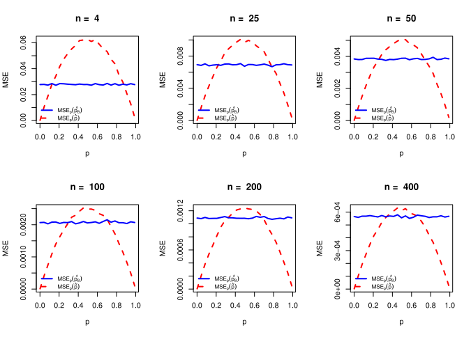
R Code for Figure 2.5
par(mfrow = c(2,3))
n_vals = c(4, 25, 50, 100, 200, 400)  # size of the sample
rep = 10^4   # number of replication
P = seq(0.001, 0.99, length.out = 25) # values of the true probability
for(n in n_vals){
  alpha = sqrt(n/4); beta = sqrt(n/4) # Beta(alpha, beta) to make the MSE constant
  mse_p_cap = numeric(length = length(P))
  mse_pB_cap = numeric(length = length(P))

  for(i in 1:length(P)){
    p_cap = numeric(rep)
    pB_cap = numeric(rep)

    for(j in 1:rep){
      d = rbinom(n, 1, P[i])
      p_cap[j] = sum(d)/n
      pB_cap[j] = (sum(d) + alpha)/(alpha + beta + n )
    }
    mse_p_cap[i] = mean((p_cap - P[i])^2)
    mse_pB_cap[i] = mean((pB_cap - P[i])^2)
  }
  ylim = c(min(mse_p_cap, mse_pB_cap), max(mse_p_cap, mse_pB_cap))
  plot(P, mse_p_cap, col = "red", lwd=2, main = paste("n = ", n),
       ylim = ylim, type = "l", ylab = "MSE", lty =2, xlab = expression(p))
  lines(P, mse_pB_cap, col = "blue", lwd=2, lty=1)
  legend = c(expression(paste("MSE"[p], (hat(p[B])))),
    expression(paste("MSE"[p], (hat(p)))))
  legend("bottomleft", legend = legend, lwd=c(2,2), col = c("blue", "red"),
    bty = "n", lty = c(1,2), cex = 0.8)
2.4 Example - IV (Generalization of Hierarchical Bayes)
We examine a generalization of the Hierarchical Bayes model. Let \(X_1, X_2, \cdots, X_n\) be an observed random sample of size \(n\) such that \[\begin{equation*} X_i|\lambda_i \sim \mbox{Poisson}(\lambda_i),~~~~~ i=1,2,\cdots,n,~~\mbox{independent}. \end{equation*}\] Suppose \(\lambda_i, ~i=1,2,\cdots,n\) have a \(\mathrm{gamma}(\alpha,\beta)\) distribution, which is the conjugate family for Poisson. So, the hierarchical model is given by, \[\begin{eqnarray*} % \nonumber to remove numbering (before each equation) X_i|\lambda_i & \sim& \mbox{Poisson}(\lambda_i),~~~~~ i=1,2,\cdots,n,~~\mbox{independent}, \\ \lambda_i &\sim& \mbox{gamma}(\alpha,\beta),~~~ i=1,2,\cdots,n,~~\mbox{independent}, \end{eqnarray*}\] where \(\alpha\) and \(\beta\) are known positive constants, usually provided by the experimenter. Our interest is to estimate the \(\lambda_i,~i=1,2,\cdots,n,\) based on observed sample. The prior distribution of \(\lambda_i\) is given by, \[\begin{equation*} \pi(\lambda_i)=\frac{e^{-\frac{\lambda_i}{\beta}}\lambda_i^{\alpha -1}}{\Gamma(\alpha) \beta^\alpha},\ i=1,2,\cdots,n. \end{equation*}\] Suppose, we have a situation where the parameter \(\beta\) is not provided by the experimenter. However, the value of \(\alpha\) is known. To obtain an estimate of \(\lambda_i\), we first have to estimate the parameter \(\beta\). A critical point is that if we would like to estimate \(\beta\), then we require independent observations from the \(\mbox{gamma}(\alpha, \beta)\) distribution. Although \(\lambda_i\)’s are there from the said distribution, but these are not observable quantities. The empirical Bayes analysis makes use of the observed sample \(X_1, X_2,\cdots, X_n\) to estimate the parameters of the prior distribution. We First obtain the marginal distribution of \(X_i\)’s. The use of moment generating function ease the process of computing the marginal distribution greatly. Let \(M_{X_i}(t) = \mbox{E}(e^{tX_i})\), be the mgf of \(X_i,~i=1,2,\cdots,n\), which is
\[\begin{eqnarray*} % \nonumber to remove numbering (before each equation) M_{X_i}(t) &=& \mbox{E}\left(e^{tX_i}\right) \\ &=& \mbox{E}\left[\mbox{E}\left(e^{tX_i}|\lambda_i\right)\right]\\ &=& \mbox{E}\left(e^{\lambda_i(e^t - 1)}\right) \\ &=& \frac{1}{\left[1 - \beta(e^t-1)\right]^{\alpha}},~~~~~~\left[M_{\lambda_i}(t) = (1-\beta t)^{-\alpha}\right]\\ &=& \left(\frac{\frac{1}{\beta+1}}{1 - \frac{\beta}{\beta+1}e^t}\right)^{\alpha}. \end{eqnarray*}\]which is the mgf of Negative Binomial distribution with parameter \(r= \alpha\) and \(p=\frac{1}{\beta+1}\). Recall that if \(X\) follows negative binomial distribution, \(X\sim \mbox{NB}(r,p)\) then mgf of \(X\) is given by \(\left(\frac{p}{1-(1-p)e^t} \right)^\alpha\) and \(\mbox{E}X = \frac{r(1-p)}{p^2}\) and \(\mbox{Var}(X) = \frac{r(1-p)}{p^2}\). So, \(X_i \sim \mbox{NB}\left( \alpha,\frac{1}{\beta+1}\right),~i=1,2,\cdots,n\), whose pmf of is given by,
\[P(X_i=x_i)=\binom{x_i +\alpha-1}{x_i}\left(\frac{1}{\beta +1}\right)^{\alpha}\left(\frac{\beta}{\beta +1}\right)^{x_i}, ~x_i\in\{0,1,2,\cdots\}.\]
A pleasant surprise is that we observe \(X_1,X_2,\cdots,X_n\) which are marginally iid and follows \(\mathrm{NB}\left(\alpha,\frac{1}{\beta +1}\right)\). Hence, \(\beta\) can be estimated by using \(X_1,X_2,\cdots,X_n\). We can use the maximum likelihood estimation method to estimate \(\beta\). The likelihood function \(\mathcal{L}(\beta)\) is given as follows;
\[\mathcal{L}(\beta)=\left[\prod_{i=1}^{n} \binom{x_i +\alpha-1}{x_i}\right]\left(\frac{1}{\beta +1}\right)^{\alpha}\left(\frac{\beta}{\beta +1}\right)^{x_i}, \tag{2.3}\]
and the corresponding log-likelihood function, \(l(\beta) = \ln (\mathcal{L}(\beta))\) is
\[ l(\beta)=\sum_{i=1}^{n}\ln \binom{x_i +\alpha-1}{x_i}-n\alpha\ln(1+\beta)+\sum_{i=1}^{n}x_i\ln\left(\frac{\beta}{1+\beta}\right). \tag{2.4}\]
Taking first order derivative with respect to \(\beta\) and making \(\frac{\partial l(\beta)}{\partial \beta}=0\), we obtain the likelihood equation as
\[\begin{equation*} \frac{-n\alpha}{1+\beta} + \left(\sum_{i=1}^{n}x_i\right)\left(\frac{1}{\beta}-\frac{1}{1+\beta}\right)=0. \end{equation*}\]On simplifying we get estimator for prior parameter \(\beta\) as, \(\hat{\beta}=\frac{\bar{\mathrm{X}}}{\alpha}\). It can be easily verified that \(\frac{\partial^2 l(\beta)}{\partial \beta^2}=\frac{n\alpha}{(\beta+1)^2}+\sum_{i=1}^{n}x_i\left(-\frac{1}{\beta^2}+\frac{1}{(1+\beta)^2}\right)\) at \(\beta=\hat{\beta}\), \(\frac{\partial^2(\beta)}{\partial \beta^2}\bigg|_{\beta=\frac{\bar{\mathrm{X}}}{\alpha}}=\frac{-n\alpha^3 \bar{\mathrm{x}}-n\alpha^4}{ \bar{\mathrm{x}}(\bar{x}+\alpha)^2} < 0\), showing that \(\hat{\beta}\) is the MLE of \(\beta\). Once the estimate of the unknown prior \(\beta\) is obtained, the model becomes
\[\begin{eqnarray*} % \nonumber to remove numbering (before each equation) X_i|\lambda_i &\Large\sim& \mbox{Poisson}(\lambda_i), ~~~~~~i=1,2,\cdots,n,~~\mbox{independent}, \\ \lambda_i &\Large\sim& \mbox{gamma}(\alpha,\hat{\beta}),~~~~~ i=1,2,\cdots,n,~~\mbox{independent}. \end{eqnarray*}\]The posterior distribution that is the conditional distribution of \(\lambda_i\) given the sample \(x_i, i=1,2,\cdots,n\) is
\[\begin{eqnarray*} \pi(\lambda_i|x_i)&=&\frac{f(x_i|\lambda_i)\pi(\lambda_i)}{f(x_i)}\\ &=&\frac{\frac{e^{-\lambda_i}\lambda_i^{x_i}}{x_i!}\frac{e^{-\frac{\lambda_i}{\hat{\beta}}}\lambda_i^{\alpha-1}}{\Gamma(\alpha) \hat{\beta}^\alpha}}{\binom{x_i +\alpha-1}{x_i}\left(\frac{1}{\hat{\beta}+1}\right)^\alpha \left(\frac{\hat{\beta}}{\hat{\beta}+1}\right)^{x_i}}\\ &=& \frac{\lambda_i^{x_i+\alpha-1}e^{-\lambda_i\left(1+\frac{1}{\hat{\beta}}\right)}\left(1+\frac{1}{\hat{\beta}}\right)^{x_i+\alpha}}{\Gamma(x_i+\alpha)}. \end{eqnarray*}\]So, \(\lambda_i|x_i\sim \mbox{gamma}\left(x_i+\alpha,\left(1+\frac{1}{\hat{\beta}}\right)^{-1}\right)\). The Bayes estimator of \(\lambda_i\) under a squared error loss, that is the posterior mean \(\mbox{E}(\lambda_i|x_i)\) is given by,
\[\begin{equation*} \hat{\lambda_i}_B=(x_i+\alpha)\left(1+\frac{1}{\hat{\beta}}\right)^{-1}. \end{equation*}\]Note that the Bayes estimate of \(\lambda_i\) contains the term \(\hat{\beta}\), which was estimated from data. Hence, there is uncertainty associated with the estimate of the prior parameter \(\beta\). We can estimate \(\mbox{Var}(\hat{\beta})\) as follows:
\[\mbox{Var}(\hat{\beta}) = \frac{1}{\alpha^2n^2}\mbox{Var}_{\beta}(\sum_{i=1}^n X_i) = \frac{1}{\alpha^2n}\mbox{Var}_{\beta}(X_1) = \frac{1}{\alpha^2n}\frac{\alpha \left(1-\frac{1}{\beta+1}\right)}{\left(\frac{1}{\beta+1}\right)^2} = \frac{\beta (\beta+1)}{n\alpha}.\]
So the estimated variance is \(\frac{\hat{\beta} (\hat{\beta}+1)}{n\alpha}\). However, it does not play any role in empirical Bayes estimation. This is a drawback of the empirical Bayes estimation. However, in hierarchical Bayes, the unknown prior parameter is replaced by a distribution. Hence the uncertainty in the hyperparameters gets included in the final estimation of the posterior mean. This is an advantage of hierarchical Bayes over empirical Bayes. The hierarchical formulation of the same problem may be stated as follows:
\[\begin{eqnarray*} % \nonumber to remove numbering (before each equation) X_i|\lambda_i &\sim & \mbox{Poisson}(\lambda_i),~~~~~i=1,2,\cdots,n,~~~\mbox{independent} \\ \lambda_i &\sim & \mbox{gamma}(\alpha,\beta),~~~ i=1,2,\cdots,n,~~~\mbox{independent}, \\ \beta &\sim & \mbox{uniform}(0,\infty)~~(\mbox{noninformative prior}). \end{eqnarray*}\] Coming back to the problem again, the empirical Bayes estimator is given by \[\begin{equation*} \hat{\lambda_i}_B = \left(\frac{\hat{\beta}}{1+\hat{\beta}}\right)x_i + \left(\frac{1}{1+\hat{\beta}}\right)(\alpha \hat{\beta}). \end{equation*}\]
Again with no surprise, \(\hat{\lambda_i}_B\) is a linear combination of the prior mean and sample mean. In above, we estimate \(\lambda_i\) using only single observation form \(\mbox{Poission}(\lambda_i),~ i=1,2,\cdots,n\). In the discussed example, we have assumed \(\alpha\) to be known and \(\beta\) unknown. However, it might happen that both \(\alpha\) and \(\beta\) are known. In such situation, both \(\alpha\) and \(\beta\) may be estimated from the observed samples \(X_1,X_2,\cdots, X_n\), whose marginal distributions are iid \(\mbox{NB}\left(\alpha, \frac{1}{\beta+1}\right)\). The likelihood equations are given by
\[\frac{\partial l(\alpha, \beta)}{\partial \alpha} = 0, ~ \frac{\partial l(\alpha, \beta)}{\partial \beta}=0,\]
where the log-likelihood function \(l(\alpha, \beta)\) is same as given in the equation Equation 2.4. These maximization must be carried out using some numerical procedures, for example Newton Raphson method. The estimates and associated standard errors can be obtained using R. For example, the likelihood function can be passed in the \(\texttt{optim}\) function or the function \(\texttt{fitdistr}\), available in the \(\texttt{MASS}\) package (Venables and Ripley 2002), may be utilized. Sample code is given below:
> x = rgamma(n = 50, shape = 2, rate = 3)
> library(MASS)
> fit = fitdistr(x = x, "gamma", lower = 0.01)
> fit$estimate
   shape     rate
1.615070 2.922565
> fit$sd
    shape      rate
0.2956650 0.6261151
> hist(x, prob = T, col = "lightgrey")
> curve(dgamma(x, shape = fit$estimate[1], rate = fit$estimate[2]),
    col = "red", lwd=2, add = TRUE)
In the same example, we may have a one way classification with \(n\) groups and \(m\) observations per group. Then the example extends to \[\begin{eqnarray*} % \nonumber to remove numbering (before each equation) X_{ij} |\lambda_i &\sim& \mbox{Poisson}(\lambda_i),~~~i=1,2,\cdots,n;~j=1,2,\cdots,m;~~~\mbox{independent}, \\ \lambda_i &\sim& \mbox{gamma}(\alpha, \beta),~~~i=1,2,\cdots,n;~~~~\mbox{independent}. \end{eqnarray*}\] To estimate \(\lambda_i\), we use the statistic \(Y_i=\sum_{j=1}^{m}X_{ij}\), then \(Y_i|\lambda_i \sim \mbox{Poisson}(m\lambda_i),~ i=1,2,\cdots,n\). The marginal pdf of \(Y_i\) is \[\begin{eqnarray*} f(y_i)&=&\int_{0}^{\infty}f(y_i|\lambda_i)\pi(\lambda_i)\mathrm{d}\lambda_i\\ &=&\int_{0}^{\infty}\frac{e^{-m\lambda_i}(m\lambda_i)^{y_i}}{y_i!}\frac{e^{-\frac{\lambda_i}{\hat{\beta}}}\lambda_i^{\alpha-1}}{\Gamma(\alpha) \hat{\beta}^\alpha}\mathrm{d}\lambda_i\\ &=&\int_{0}^{\infty}\frac{e^{-\lambda_i\left(m+\frac{1}{\beta}\right)}m^{y_i}\lambda_i^{y_i+\alpha-1}}{y_i!\beta^{\alpha}\Gamma(\alpha)}\\ &=&\frac{m^{y_i}\left\lbrace\left(m+\frac{1}{\beta}\right)^{-1}\right\rbrace^{y_i+\alpha}\Gamma(y_i+\alpha)}{y_i!\beta^{\alpha}\Gamma(\alpha)}\\ &=&\frac{\Gamma(y_i+\alpha+1-1)}{\Gamma(y_i+1)\Gamma(\alpha)}\left(\frac{m\beta}{m\beta+1}\right)^{y_i}\left(\frac{1}{m\beta+1}\right)^\alpha\\ &=&\binom{y_i +\alpha-1}{y_i}\left(\frac{1}{m\beta+1}\right)^\alpha\left(1-\frac{1}{m\beta+1})\right)^{y_i}. \end{eqnarray*}\] So, \(Y_i\sim \mbox{NB}\left(\alpha,\frac{1}{m\beta+1}\right),~ i=1,2,\cdots,n\). The posterior distribution of \(\lambda_i\) is given by, \[\begin{eqnarray*} \pi(\lambda_i|y_i)&=&\frac{f(y_i|\lambda_i)\pi(\lambda_i)}{f(y_i)}\\ &=&\frac{\frac{e^{m\lambda_i}(m \lambda_i)^{y_i}}{y_i!}\frac{e^{-\frac{\lambda_i}{\beta}}\lambda_i^{\alpha-1}}{\beta^{\alpha}\Gamma(\alpha)}}{f(y_i)}\\ &=&\frac{\lambda_i^{y_i+\alpha-1}e^{-\lambda_i\left(m+\frac{1}{\beta}\right)}\left(m+\frac{1}{\beta}\right)^{y_i+\alpha}}{\Gamma(y_i+\alpha)}, \end{eqnarray*}\] which shows that \(\lambda_i|y_i \sim \mbox{gamma}\left(y_i+\alpha,\left(m+\frac{1}{\beta}\right)^{-1}\right)\). The posterior mean, that is the Bayes estimator of \(\lambda_i\) under a squared error loss is \[\begin{eqnarray*} \hat{\lambda_i}_B&=& \mbox{E}(\lambda_i|y_i)\\ &=&(y_i+\alpha)\left(m+\frac{1}{\beta}\right)^{-1}\\ &=&\left(\sum_{j=1}^{m}x_{ij} +\alpha\right) \left(m+\frac{1}{\beta}\right)^{-1},\\ &=&\left(\frac{m\beta}{1+m\beta}\right)\bar{X_i} + \left(\frac{1}{1+m\beta}\right)(\alpha \beta). \end{eqnarray*}\] Thus, \(\hat{\lambda_i}_B\) is a linear combination of the prior mean and sample mean. The variance of \(\hat{\lambda_i}_B\) is given by \[\begin{eqnarray*} \mbox{Var}_{\lambda_i}(\hat{\lambda_i}_B)&=&\left(\frac{m\beta}{1+m\beta}\right)^2\mbox{Var}_{\lambda_i}(\bar{X_i}),\\ &=& \left(\frac{m\beta}{1+m\beta}\right)^2\left(\frac{\lambda_i}{m}\right). \end{eqnarray*}\] With no surprise, for large \(m\), the above expression is close to the variance of maximum likelihood estimator \(\left(\frac{m\beta}{m\beta + 1} \to 1 \mbox{ for large } m\right)\).
2.5 Example - V (Gamma prior for Exponential rate parameter)
Let \(Y_1\),\(Y_2\),\(\cdots\),\(Y_n\) be a observed random sample of size \(n\) such that \[\begin{equation*} Y_i|\lambda \sim \mbox{exponential}(\lambda),\ i=1,2,\cdots,n,~~\mbox{independent}. \end{equation*}\] Suppose that \(\lambda\) has a \(\mbox{gamma}(\alpha,\beta)\) distribution, which is the conjugate family for Exponential. So, the statistical model has the following hierarchy
\[\begin{eqnarray} Y_i|\lambda &\sim& \mbox{exponential}(\lambda),\ i=1,2,\cdots,n,\\ \lambda &\sim& \mbox{gamma}(\alpha,\beta), \end{eqnarray}\]
where \(\alpha\) and \(\beta\) are known. Now, our interest is to estimate the \(\lambda\) based on observed sample. The prior distribution of \(\lambda\) is given by,
\[\begin{equation} \pi(\lambda)=\frac{e^{-\frac{\lambda}{\beta}}\lambda^{\alpha -1}}{\Gamma(\alpha)\beta^\alpha }, \lambda>0, \end{equation}\]
where \(\alpha\) and \(\beta\) are positive constants. First, we shall estimate the posterior distribution of \(\lambda\). We start with statistic \(Z\) = \(\sum_{i=1}^n Y_i\). Sampling distribution of \(Z\) is \(\mbox{gamma}(n,\lambda)\) and it is denoted by \(f(z|\lambda).\) The posterior distribution of \(\lambda\) given the sample \(Y_1,Y_2,\cdots,Y_n\), that is given \(Z = z,\) is
\[\begin{equation*} \pi(\lambda|z) = \frac{f(z|\lambda)\pi(\lambda)}{f(z)}, \end{equation*}\]
where \(f(z)\) is the marginal distribution of \(Z\), and calculated as follows;
\[\begin{eqnarray*} f(z) &=& \int_{0}^{\infty}f(z|\lambda)\pi(\lambda) \mathrm{d}\lambda \\ &=& \int_{0}^{\infty} \frac{z^{n-1}e^{-\lambda z}\lambda^n}{\Gamma(n)}\frac{\lambda^{\alpha-1}e^{-\frac{\lambda}{\beta}}}{\Gamma(\alpha)\beta^\alpha} \mathrm{d}\lambda \\ &=& \frac{z^{n-1}}{\Gamma(n)\Gamma(\alpha)\beta^\alpha}\int_{0}^{\infty} e^{-\lambda(z+\frac{1}{\beta})} \lambda^{\alpha+n-1} \mathrm{d}\lambda \\ &=& \frac{z^{n-1} \Gamma(\alpha + n)}{\Gamma(n)\Gamma(\alpha)\beta^\alpha (z+\frac{1}{\beta})^{\alpha+n}} \int_{0}^{\infty} \frac{\lambda^{\alpha+n-1}e^{-\lambda(z+ \frac{1}{\beta})}(z+\frac{1}{\beta})^{\alpha+n}}{\Gamma(\alpha+n)} \mathrm{d}\lambda \\ &=& \frac{ z^{n-1} \Gamma(\alpha + n)}{\Gamma(n)\Gamma(\alpha)\beta^\alpha (z+\frac{1}{\beta})^{\alpha+n}}, \end{eqnarray*}\] where,\[\begin{equation*} \int_{0}^{\infty} \frac{\lambda^{\alpha+n-1}e^{-\lambda(z+\frac{1}{\beta})}(z+\frac{1}{\beta})^{\alpha+n}}{\Gamma(\alpha+n)} \,d\lambda = 1. \end{equation*}\]
because it is pdf of \(\mbox{gamma}\left(\alpha+n,(z+\frac{1}{\beta})^{-1}\right)\) distribution. So integral reduces to 1. Now, posterior density \(\pi(\lambda|z)\) becomes,
\[\begin{eqnarray*} \pi(\lambda|z) &=& \frac{f(z|\lambda)\pi(\lambda)}{f(z)} \\ &=& \frac{z^{n-1}e^{-\lambda z}\lambda^n}{\Gamma(n)}\frac{e^{-\frac{\lambda}{\beta}}\lambda^{\alpha -1}}{\Gamma(\alpha)\beta^\alpha}\frac{\Gamma(n)\Gamma(\alpha)(z+\frac{1}{\beta})^{\alpha+n}\beta^\alpha}{ z^{n-1}\Gamma(\alpha+n)} \\ &=& \frac{e^{-\lambda(z+\frac{1}{\beta})}\lambda^{\alpha+n-1}(z+\frac{1}{\beta})^{\alpha+n}}{\Gamma(\alpha+n)}, 0<\lambda<\infty. \end{eqnarray*}\]
Hence, the posterior distribution of \(\lambda\), \(\lambda|z\sim \mbox{gamma}\left(\alpha+n,(z+\frac{1}{\beta})^{-1}\right)\). So exact posterior mean \(\mbox{E}(\lambda|z)\) is \[\begin{equation*} \frac{\alpha+n}{z+\frac{1}{\beta}} = \frac{\alpha+n}{n\bar{y}+\frac{1}{\beta}} \end{equation*}\] Now, we approximate the posterior mean of \(\lambda\) using a Monte Carlo (MC) sample, given \(m\) independent values drawn directly from \(\mbox{gamma}(\alpha+n,n\bar{y}+\frac{1}{\beta})\) posterior distribution. Further, the accuracy of the monte carlo approximation is compared with respect to the exact posterior distribution. First of all, we generated \(y\) of size \(n=50\) from exponential distribution with parameter \(\lambda\), where \(\lambda\) was generated from \(\mbox{gamma}(\alpha = 8,\beta = 4)\) density function. To generate the independent values of \(\lambda\) of the MC sample from the known posterior distribution the function \(\texttt{rgamma}\) was utilized with posterior rate and shape parameter.
R Code for Figure 2.6
set.seed(123)
n = 50                                          # sample size
alpha = 8                                       # prior parameter
beta = 4                                        # prior parameter
lambda = rgamma(1,alpha,beta)                   # true lambda
lambda
y = rexp(n = n,rate = lambda)                   # data (simulated here)
p_alpha = alpha + n; p_alpha                    # posterior alpha
p_beta = (1/beta) + n*mean(y); p_beta           # posterior beta
p_mean = p_alpha/p_beta; p_mean                 # exact posterior mean
par(mfrow=c(1,3))
M = c(100,500,1000)
for (m in M) {
  z1 = rgamma(n=m, shape=p_alpha, rate=p_beta)
  hist(z1, probability = TRUE,main=paste("m =",m),
       xlab=expression(lambda),col = "light grey", cex.lab = 1.5, cex.main = 1.5)
  curve(dgamma(x, shape = p_alpha, rate = p_beta),
        col ="blue", add=TRUE, lwd = 2)
  points(lambda, 0, pch = 19,col = "red", cex = 2)}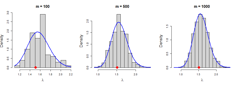
2.6 Exercises
(Casella and Berger 2002) If \(S^2\) is the sample variance based on a sample of size \(n\) from a normal population, we know that \((n-1)S^2/\sigma^2\) has a \(\chi_{n-1}^2\) distribution. The conjugate prior for \(\sigma^2\) is the inverted gamma pdf, IG(\(\alpha, \beta\)), given by, \[\begin{equation*} \pi(\sigma^2) = \frac{1}{\Gamma(\alpha)\beta^{\alpha}}\frac{1}{\left(\sigma^2 \right)^{\alpha+1}}e^{-1/(\beta \sigma^2)},~~0<\sigma^2 <\infty, \end{equation*}\] where \(\alpha\) and \(\beta\) are positive constants. Show that the posterior distribution of \(\sigma^2\) is \[\begin{equation*} \mbox{IG}\left(\alpha+\frac{n-1}{2}, \left[\frac{(n-1)S^2}{2} + \frac{1}{\beta}\right]^{-1}\right). \end{equation*}\]
Find the mean of this distribution, the Bayes estimator of \(\sigma^2\).
Suppose that \(X_1, X_2,\cdots, X_n\) is a random sample from the distribution with pdf \[\begin{eqnarray*} % \nonumber to remove numbering (before each equation) f(x|\theta) &=& \theta x^{\theta - 1},~~~0 < x<1, \\ &=& 0,~~~~~~~~\mbox{otherwise}. \end{eqnarray*}\] Suppose also that the value of the parameter \(\theta\) is unknown (\(\theta>0\)) and that the prior distribution of \(\theta\) is \(\mbox{gamma}(\alpha, \beta)\), \(\alpha >0\) and \(\beta>0\). Determine the posterior distribution of \(\theta\) and hence obtain the Bayes estimator of \(\theta\) under a squared error loss function.
(Casella and Berger 2002) Suppose that we observe \(X_1, X_2,\cdots, X_n\) where \[\begin{eqnarray*} % \nonumber to remove numbering (before each equation) X_i|\theta_i &\sim & \mathcal{N}(\theta_i, \sigma^2),~~i=1, 2,\cdots,n, ~~~\mbox{independent}\\ \theta_i &\sim & \mathcal{N}(\mu,\tau^2),~~~i=1, 2,\cdots,n, ~~~\mbox{independent} \end{eqnarray*}\]
- Show that the marginal distribution of \(X_i\) is \(\mathcal{N}(\mu, \sigma^2)\) and that, marginally, \(X_1, X_2,\cdots,X_n\) are iid. Empirical Bayes analysis would use the marginal distribution of \(X_i\)’s to estimate the prior parameters \(\mu\) and \(\tau^2\).
- Show, in general, that if \[\begin{eqnarray*} % \nonumber to remove numbering (before each equation) X_i|\theta_i &\sim & f(\theta_i, \sigma^2),~~i=1, 2,\cdots,n, ~~~\mbox{independent}\\ \theta_i &\sim & \pi(\theta|\tau),~~~~i=1, 2,\cdots,n, ~~~\mbox{independent} \end{eqnarray*}\] then \(X_1, X_2,\cdots,X_n\) are iid.
(Wasserman 2004) Suppose that we observe \(X_1, X_2,\cdots, X_n\) from \(\mathcal{\mu, 1}\). (a)Simulate a data set (using \(\mu=5\)) consisting of \(n=100\) observations. (b)Take \(\pi(\mu)=1\) and find the posterior density and plot the density. (c)Simulate 1000 draws from the posterior and plot the histogram of the simulated values and compare the histogram to the answer in (b). (d)Let \(\theta= \exp(\mu)\), then find the posterior density for \(\theta\) analytically and by simulation. (e)Obtain a 95 percent posterior interval for \(\mu\) and \(\theta\).
(Wasserman 2004) Consider the Bernoulli(\(p\)) observations: \[0~1~0~1~0~0~0~0~0~0\] Plot the posterior for \(p\) using these prior distributions for \(p\): \(\mbox{beta}(1/2, 1/2)\), \(\mbox{beta}(10, 10)\) and \(\mbox{beta}(100, 100)\).
(Wasserman 2004) Let \(X_1, X_2,\cdots,X_n \sim \mbox{Poisson}(\lambda)\). Find the Jeffrey’s prior. Also, find the corresponding posterior density function.